
Introduction to Machine Learning in Python
Graduate course lecture, University of Toronto Missisauga, Department of Chemical and Physical Sciences, 2019
These lecture and practical are created for CPS Teaching Fellowship where we introduce a novel approach to study advanced scientific programming. The goal of the lecture is to introduce Machine Learning (ML) tools and how to use them for Molecular Dynamics simulations in Python programmming language. We will use a lot of numpy functions and a few of new modules, such as sklearn for dimensionality reduction. Lecture on github
Important concepts that we will cover:
Lecture:
- Supervised and unsupervised machine learning
- Dimensionality reduction
- Principal Component Analysis (PCA)
- Multidimensional Scaling (MDS)
Practical:
- Application of PCA to MD simulations to study folding
- Application of MDS to build the Old World Map
Lecture 9: Introduction to Machine Learning in Python
1. Introduction
This lecture was created as part of a CPS Teaching Fellowship. We are introducing a novel approach to study advanced scientific programming. The goal of today’s lecture is to present unsupervised Machine Learning. We will learn about the most typical machine learning problems, such as dimensionality reduction, and how to approach these using the Python programmming language. These are the important concepts that we will cover:
- Machine Learning
- Data sets
- Dimensionality reduction
- Principal Component Analysis (PCA)
- Multidimensional Scaling (MDS)
- Other dimensionality reduction techniques
2. Machine Learning
Below is the outline of the field with specific algorithms:
- Unsupervised Learning - there is no correct input/output pair
- Clustering
- K-Means
- Hierarchical
- Spectral
- Dimensionality reduction
- Principal Components Analysis (PCA)
- Multidimensional Scaling (MDS)
- Stochastic Neighbour Embedding (t-SNE)
- Uniform Manifold Approximation and Projection (UMAP)
- Clustering
- Supervised Learning - there is a correct input/output pair
- Regression
- Curve fitting
- Linear regression
- Classification
- Linear Classifiers (Support Vector Machines, Logistic regression)
- Decision Trees
- Neural Networks
- Regression
- Reinforcement Learning - is an area concerned with how software agents have to take actions in an environment so as to maximize some cumulative reward
3. Generating data sets
Setup:
- Suppose one has $p$ samples of N-dimensional data points, $x_i\in\mathbb{R}^N$
- Store these samples columnwise as $X\in\mathbb{R}^{p\,\times\,N}$
- We call this the original data matrix, or simply the data
- Assumption: there is a meaningful metric (e.g. Euclidean distance) on the data space (high dim)
- Assumption: there is a meaningful metric (e.g. Euclidean distance) on the latent space (low dim)
import numpy as np
import matplotlib.pyplot as plt

plt.style.use('seaborn-darkgrid')
Generate linear data with noise ( 2-dimensional data set):
plt.style.use('seaborn-poster')

raw_data_x = np.random.uniform(0,10, size=(100,))
raw_data_y = 0.5 * raw_data_x + np.random.normal(0,1,len(raw_data_x))

X_2d = np.empty((100, 2))
X_2d[:,0] = raw_data_x
X_2d[:,1] = raw_data_y

#plt.figure(figsize=(12,8))
plt.scatter(X_2d[:,0], X_2d[:,1])
plt.xlim(-1, 11)
plt.ylim(-2, 7.2)
plt.show()
Let’s look how the data looks like (first 10 points):
X_2d[:10]
Load some high-dimensional data from the MNIST dataset. 
from keras.datasets import mnist
(x_train, y_train), (x_test, y_test) = mnist.load_data()
x_train.shape, x_test.shape, y_train.shape, y_test.shape
Let’s take only 1000 data points
X = x_test[:1000]
Y = y_test[:1000]
plt.imshow(X[567], cmap='gray')
plt.show()
We want to convert each data point (picture with a handwritten digit) to a vector which dimensionality is 28x28 = 784
X = X.reshape(1000, 784)
X[567].shape
Summary - we have two data sets:
- Two-dimensional data set with 100 points
- 768-dimensional data set with 1000 points
4. Dimensionality reduction
Dimensionality reduction is the process of reducing the number of dimensions under consideration by obtaining a set of principal variables. You can select a subset of original variables, or find a linear or nonlinear combination of features, or make a projection to lower dimensions.

Methods:
- Principal Components Analysis (PCA) - linear method to extract dimensions with the highest variance
- Multidimensional Scaling (MDS) - nonlinear method to project in lower dimensions by saving pairwise distances
- Stochastic Neighbour Embedding (t-SNE) - making an embedding in lower dimensions by conserving distribution of distances
- Uniform Manifold Approximation and Projection (UMAP) - projecting the data on manifold into fewer dimensions
5. Principal Component Analysis
Math:
- PCA goal: Find orthogonal transformation $W$ of centered data $X_c$ (i.e. $Y=WX_c$) such that variance along subsequent components is maximized (i.e. most variance along first, etc.); note $X_c$ is $p \times N$, $W$ is $N \times N$, $Y$ is $p \times N$, principal components are the columns of $W$
- principal components of $X_c$ are typically found via eigendecomposition of covariance matrix $X_c^T X_c$
- the PCA embedding is $Y=U^T X_c$, where $U$ stores columnwise eigenvectors of $X_c^T X_c$ in decreasing order (by eigenvalue)
Compute principle components via eigenvectors of covariance matrix
- Center data, i.e. first subtract the mean from the data
- Compute the covariance matrix
- Compute eigenvectors and order them in terms of decreasing eigenvalues
- Transform the data using these eigenvectors
- Compare to library PCA implementation
# For data set # 1:

# step 1
X_2d_centered = X_2d - np.mean(X_2d, axis=0)
plt.scatter(X_2d_centered[:,0], X_2d_centered[:,1])
plt.ylim((-4,4))
plt.xlim((-6,6))
plt.show()
We see that the data is now centered on the origin. Now compute the transformation:
# Step 2.
Cov = np.dot(np.transpose(X_2d_centered), X_2d_centered)
print("Covariance matrix:")
print(Cov)

#Step 3
Eigvals, W = np.linalg.eig(Cov)
print("\nEigenvalues:")
print(Eigvals)
print("\nEigenvectors (columns)")
print(W)
print("\nCheck that eigenvectors are orthogonal (<w1,w2>=0):")
print(np.dot(W[:,0],W[:,1]))

print('\nVarience in the first principal component: {}, varience in the second principal component: {}'.format(Eigvals[0]/np.sum(Eigvals), Eigvals[1]/np.sum(Eigvals) ))
Let’s plot the eigenvectors in comparison to the data
plt.scatter(X_2d_centered[:,0], X_2d_centered[:,1])
plt.plot([0, W[0][1]*3],[0, W[1][1]*3],'r',linewidth=4)
plt.plot([0, W[0][0]*5],[0, W[1][0]*5],'g',linewidth=4)
plt.ylim((-6,6))
plt.xlim((-8,8))
plt.show()
Now we will apply the transformation to the data and plot the data in the new space. We flip the matrix W and corresponding eigenvalues so that they are ordered the same way as in the theory.
#Step 4
#W = np.fliplr(W)
Eigvals = Eigvals[::-1]
X_2d_transformed = np.dot(X_2d_centered, W)
plt.scatter(X_2d_transformed[:,0], X_2d_transformed[:,1])
plt.ylim((-6,6))
plt.xlim((-8,8))
plt.xlabel('PC 1')
plt.ylabel('PC 2')
plt.show()
Let’s compare our naive implementation to the PCA implementation from sklearn
from sklearn.decomposition import PCA

skl_PCA = PCA(n_components = 2).fit(X_2d) ## fit the data to receive eigenvectors of covariance matrix
skl_X_2d_transformed = skl_PCA.transform(X_2d) ## apply a transformation

plt.scatter(skl_X_2d_transformed[:,0], skl_X_2d_transformed[:,1])
plt.xlabel('PC 1')
plt.ylabel('PC 2')
plt.ylim((-6,6))
plt.xlim((-8,8))
plt.show()
Looks identical (up to a left-right or up-down flip)!
We will now truncate the data to one dimension and see how it looks. It’s called a simple PCA dimensionality reduction.
print(skl_PCA.explained_variance_ratio_)
We notice that >90% of variance is in the first principal component
plt.scatter(skl_X_2d_transformed[:,0] , np.zeros(shape=skl_X_2d_transformed[:,0].shape))
plt.ylim((-6,6))
plt.xlim((-8,8))
plt.show()
Exercise 5.1
Perform principal component analysis on the 1000 points of MNIST data set. It’s already contained in the memory of the Jupyter Notebook under variable X. Y contains the label of each handwritten digit, i.e. the number, or the class. Documentation on sklearn PCA
- Plot the total variance vs the number of PC. Hint: variable
explained_variance_ratio_may be useful. - Use the first two component to represent MNIST data set in two dimensions on a scatter plot.
- Show the image of first first principal eigenvector. Hint: variable
components_and functionreshape()might be useful.
6. Multidimensional Scaling (MDS)
Metric MDS
Setup:
- Suppose one has $p$ samples of N-dimensional data points, $x_i\in\mathbb{R}^N$
- Store these samples rowwise as $X\in\mathbb{R}^{p\,\times\,N}$
- We call this the original data matrix, or simply the data
- Assumption: there is a meaningful metric (e.g. Euclidean distance) on the data space (high dim)
- Assumption: there is a meaningful metric (e.g. Euclidean distance) on the latent space (low dim)
Goal:
- Given N-dim data $X$, a metric $d(\cdot,\cdot)$ on $\mathbb{R}^N$, a target dimension $k<N$, and a metric $g(\cdot,\cdot)$ on $\mathbb{R}^k$
- Find an embedding $Y\in\mathbb{R}^{k\,\times\,p}$ (i.e. a $y_i\in\mathbb{R}^k$ for each $x_i\in\mathbb{R}^N$) such that distances $d_{ij}$, $g_{ij}$ are preserved between representations
| Objective function: $$Y^\ast=\operatorname*{arg\,min}Y {\sum{i<j}{\left | d_{ij}\left(X\right)-g_{ij}\left(Y\right)\right | }}$$ |
Let’s not invent the wheel and use MDS implementation in Python:
from sklearn.manifold import MDS
from scipy.spatial.distance import pdist, squareform
# compute MDS embedding (2D)
# Docs: http://scikit-learn.org/stable/modules/generated/sklearn.manifold.MDS.html
Can we predict the outcome of MDS from 2D to 2D?
## First, we should find pairwise distances.
D_compressed = pdist(X_2d, metric='euclidean') # n*(n-1)/2 size
D = squareform(D_compressed)
D.shape
mds_2d = MDS(n_components=2, dissimilarity='precomputed', n_jobs=-1 ).fit_transform(D)
plt.scatter(mds_2d[:,0], mds_2d[:,1], color='red')
plt.ylim((-6,6))
plt.xlim((-8,8))
plt.xlabel('MDS axis 1')
plt.ylabel('MDS axis 2')
plt.show()
Restores original coordinates up to a flip…
What about high dimensional data?
mds_X = MDS(n_components=2, dissimilarity='euclidean', n_jobs=4).fit_transform(X) ## distances will be computed

plt.scatter(mds_X[:,0], mds_X[:,1], marker='.')
plt.xlabel('MDS axis 1')
plt.ylabel('MDS axis 2')
plt.show()
This is what we get as an output of the algorithm
mds_X.shape
for label in set(Y):
    mask = Y==label
    plt.scatter(mds_X[:,0][mask], mds_X[:,1][mask], marker = '.', label = label)
plt.legend()
plt.xlabel('MDS axis 1')
plt.ylabel('MDS axis 2')
plt.show()
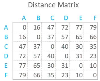
Exercise 6.1.
Find the relative coordinates (sketch of the map) of the European cities knowing only pairwise distances between them. Remember that MDS embedding may require rotation and/or horizontal and vertical flip. You should get relative locations similar to these: 
import pandas as pd
# Pairwise distance between European cities
url = 'https://raw.githubusercontent.com/neurospin/pystatsml/master/datasets/eurodist.csv'
df = pd.read_csv(url)
print(df.iloc[:7, :7])
print()
## Array with cities:
city = np.array(df["city"])

## Squareform distance matrix
D = np.array(df.iloc[:, 1:])
print(D.shape)
print()
print(city)
## Write your code here
7. Other dimensionality reduction techniques: t-SNE, UMAP
from sklearn.manifold import TSNE
import umap
t-SNE
tsne_2d = TSNE(n_components=2).fit_transform(X)

plt.scatter(tsne_2d[:,0], tsne_2d[:,1], marker='.')
plt.show()
Show with labels:
for label in set(Y):
    mask = Y==label
    plt.scatter(tsne_2d[:,0][mask], tsne_2d[:,1][mask], marker = '.', label = label)   #, color =  label + 1) #, label = str(label))
plt.legend()
plt.show()
UMAP
umap_2d = umap.UMAP(n_components=2).fit_transform(X)

plt.scatter(umap_2d[:,0], umap_2d[:,1], marker='.', color='blue')
plt.show()
Show with labels:
for label in set(Y):
    mask = Y==label
    plt.scatter(umap_2d[:,0][mask], umap_2d[:,1][mask], marker = '.', label = label)   #, color =  label + 1) #, label = str(label))
plt.legend()
plt.show()